
What is PyTorch?

PyTorch is a Torch based machine learning library for Python. It's similar to numpy but with powerful GPU support. It was developed by Facebook's AI Research Group in 2016. PyTorch offers Dynamic Computational Graph such that you can modify the graph on the go with the help of autograd. Pytorch is also faster in some cases than other frameworks, but you will discuss this later in the other section.
PyTorch Advantages and Weakness
Advantages
- Simple LibraryPyTorch code is simple. It is easy to understand, and you use the library instantly. For example, take a look at the code snippet below:
class Net(torch.nn.Module):
   def __init__(self):
       super(Net, self).__init__()
       self.layer = torch.nn.Linear(1, 1)

   def forward(self, x):
       x = self.layer(x)
       return x
As above, you can define the network model easily, and you can understand the code quickly without much training.
- Dynamic Computational Graph

Pytorch offers Dynamic Computational Graph (DAG). Computational graphs is a way to express mathematical expressions in graph models or theories such as nodes and edges. The node will do the mathematical operation, and the edge is a Tensor that will be fed into the nodes and carries the output of the node in Tensor.
DAG is a graph that holds arbitrary shape and able to do operations between different input graphs. Every iteration, a new graph is created. So, it is possible to have the same graph structure or create a new graph with a different operation, or we can call it a dynamic graph.
- Better Performance
Communities and researchers, benchmark and compare frameworks to see which one is faster. A GitHub repo Benchmark on Deep Learning Frameworks and GPUs reported that PyTorch is faster than the other framework in term of images processed per second.
As you can see below, the comparison graphs with vgg16 and resnet152


- Native Python
PyTorch is more python based. For example, if you want to train a model, you can use native control flow such as looping and recursions without the need to add more special variables or sessions to be able to run them. This is very helpful for the training process.
Pytorch also implements Imperative Programming, and it's definitely more flexible. So, it's possible to print out the tensor value in the middle of a computation process.
Weakness
PyTorch is not yet officially ready, because it is still being developed into version 1. So, further development and research is needed to achieve a stable version.
PyTorch Vs. TensorFlow

The most popular deep learning framework is Tensorflow. Developed by Google's Brain Team, it's the foremost common deep learning tool.
PyTorch vs. Tensorflow
| Parameters | PyTorch | Tensorflow |
| Model Definition | The model is defined in a subclass and offers easy to use package | The model is defined with many, and you need to understand the syntax |
| GPU Support | Yes | Yes |
| Graph Type | Dynamic | Static |
| Tools | No visualization tool | You can use Tensorboard visualization tool |
| Community | The community still growing | Large active communities |
Installing PyTorch
Linux
It's straightforward to install it in Linux. You can choose to use a virtual environment or install it directly with root access. Type this command in the terminal
pip3 install --upgrade torch torchvision
AWS Sagemaker
Sagemaker is one of the platforms in Amazon Web Service that offers a powerful Machine Learning engine with pre-installed deep learning configurations for data scientist or developers to build, train, and deploy models at any scale.
First Open the Amazon Sagemaker console and click on Create notebook instance and fill all the details for your notebook.

Next Step, Click on Open to launch your notebook instance.

Finally, In Jupyter, Click on New and choose conda_pytorch_p36 and you are ready to use your notebook instance with Pytorch installed.
PyTorch Framework Basics
Let's learn the basic concepts of PyTorch before we deep dive. PyTorch uses Tensor for every variable similar to numpy's ndarray but with GPU computation support. Here we will explain the network model, loss function, Backprop, and Optimizer.
Network Model
The network can be constructed by subclassing the torch.nn. There are 2 main parts,
- The first part is to define the parameters and layers that you will use
- The second part is the main task called the forward process that will take an input and predict the output.
Import torch
import torch.nn as nn
import torch.nn.functional as F

class Model(nn.Module):
 def __init__(self):
        super(Model, self).__init__()
        self.conv1 = nn.Conv2d(3, 20, 5)
        self.conv2 = nn.Conv2d(20, 40, 5)
self.fc1 = nn.Linear(320, 10)

def forward(self, x):
       x = F.relu(self.conv1(x))
       x = F.relu(self.conv2(x))
       x = x.view(-1, 320)
       x = F.relu(self.fc1(x))
       return F.log_softmax(x)

net = Model()
As you can see above, you create a class of nn.Module called Model. It contains 2 Conv2d layers and a Linear layer. The first conv2d layer takes an input of 3 and the output shape of 20. The second layer will take an input of 20 and will produce an output shape of 40. The last layer is a fully connected layer in the shape of 320 and will produce an output of 10.
The forward process will take an input of X and feed it to the conv1 layer and perform ReLU function,
Similarly, it will also feed the conv2 layer. After that, the x will be reshaped into (-1, 320) and feed into the final FC layer. Before you send the output, you will use the softmax activation function.
The backward process is automatically defined by autograd, so you only need to define the forward process.
Loss Function
The loss function is used to measure how well the prediction model is able to predict the expected results. PyTorch already has many standard loss functions in the torch.nn module. For example, you can use the Cross-Entropy Loss to solve a multi-class classification problem. It's easy to define the loss function and compute the losses:
loss_fn = nn.CrossEntropyLoss()

#training process
loss = loss_fn(out, target)
It's easy to use your own loss function calculation with PyTorch.
Backprop
To perform the backpropagation, you simply call the los.backward(). The error will be computed but remember to clear the existing gradient with zero_grad()
net.zero_grad() # to clear the existing gradient
loss.backward() # to perform backpropragation
Optimizer
The torch.optim provides common optimization algorithms. You can define an optimizer with a simple step:
optimizer = torch.optim.SGD(net.parameters(), lr = 0.01, momentum=0.9)
You need to pass the network model parameters and the learning rate so that at every iteration the parameters will be updated after the backprop process.
Simple Regression with PyTorch
Step 1) Creating our network model
Our network model is a simple Linear layer with an input and an output shape of 1.
from __future__ import print_function

import torch
import torch.nn as nn
import torch.nn.functional as F
from torch.autograd import Variable

class Net(nn.Module):
   def __init__(self):
       super(Net, self).__init__()
       self.layer = torch.nn.Linear(1, 1)

   def forward(self, x):
       x = self.layer(x)
       return x

net = Net()
print(net)
And the network output should be like this
Net(
  (hidden): Linear(in_features=1, out_features=1, bias=True)
)
Step 2) Test Data
Before you start the training process, you need to know our data. You make a random function to test our model. Y = x3 sin(x)+ 3x+0.8 rand(100)
# Visualize our data
import matplotlib.pyplot as plt
import numpy as np

x = np.random.rand(100)
y = np.sin(x) * np.power(x,3) + 3*x + np.random.rand(100)*0.8

plt.scatter(x, y)
plt.show()
Here is the scatter plot of our function:

Before you start the training process, you need to convert the numpy array to Variables that supported by Torch and autograd
# convert numpy array to tensor in shape of input size
x = torch.from_numpy(x.reshape(-1,1)).float()
y = torch.from_numpy(y.reshape(-1,1)).float()
print(x, y)
Step 3) Optimizer and Loss
Next, you should define the Optimizer and the Loss Function for our training process.
# Define Optimizer and Loss Function
optimizer = torch.optim.SGD(net.parameters(), lr=0.2)
loss_func = torch.nn.MSELoss()
Step 4) Training
Now let's start our training process. With an epoch of 250, you will iterate our data to find the best value for our hyperparameters.
inputs = Variable(x)
outputs = Variable(y)
for i in range(250):
   prediction = net(inputs)
   loss = loss_func(prediction, outputs)
   optimizer.zero_grad()
   loss.backward()
   optimizer.step()

   if i % 10 == 0:
       # plot and show learning process
       plt.cla()
       plt.scatter(x.data.numpy(), y.data.numpy())
       plt.plot(x.data.numpy(), prediction.data.numpy(), 'r-', lw=2)
       plt.text(0.5, 0, 'Loss=%.4f' % loss.data.numpy(), fontdict={'size': 10, 'color':  'red'})
       plt.pause(0.1)

plt.show()
Step 5) Result
As you can see below, you successfully performed regression with a neural network. Actually, on every iteration, the red line in the plot will update and change its position to fit the data. But in this picture, you only show you the final result

Image Classification with PyTorch
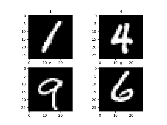
One of the popular methods to learn the basics of deep learning is with the MNIST dataset. It is the "Hello World" in deep learning. The dataset contains handwritten numbers from 0 - 9 with the total of 60,000 training samples and 10,000 test samples that are already labeled with the size of 28x28 pixels.

Step 1) Preprocess the Data
Before you start the training process, you need to understand the data. In the first step, you will load the dataset using torchvision module. Torchvision will load the dataset and transform the images with the appropriate requirement for the network such as the shape and normalizing the images.
import torch
import torchvision
import numpy as np
from torchvision import datasets, models, transforms

# This is used to transform the images to Tensor and normalize it
transform = transforms.Compose(
   [transforms.ToTensor(),
    transforms.Normalize((0.5, 0.5, 0.5), (0.5, 0.5, 0.5))])

training = torchvision.datasets.MNIST(root='./data', train=True,
                                       download=True, transform=transform)
train_loader = torch.utils.data.DataLoader(training, batch_size=4,
                                         shuffle=True, num_workers=2)

testing = torchvision.datasets.MNIST(root='./data', train=False,
                                      download=True, transform=transform)
test_loader = torch.utils.data.DataLoader(testing, batch_size=4,
                                        shuffle=False, num_workers=2)

classes = ('0', '1', '2', '3',
          '4', '5', '6', '7', '8', '9')

import matplotlib.pyplot as plt
import numpy as np

#create an iterator for train_loader
# get random training images
data_iterator = iter(train_loader)
images, labels = data_iterator.next()

#plot 4 images to visualize the data
rows = 2
columns = 2
fig=plt.figure()
for i in range(4):
   fig.add_subplot(rows, columns, i+1)
   plt.title(classes[labels[i]])
   img = images[i] / 2 + 0.5     # this is for unnormalize the image
   img = torchvision.transforms.ToPILImage()(img)
   plt.imshow(img)
plt.show()
The transform function converts the images into tensor and normalizes the value. The function torchvision.transforms.MNIST, will download the dataset (if it's not available) in the directory, set the dataset for training if necessary and do the transformation process.
To visualize the dataset, you use the data_iterator to get the next batch of images and labels. You use matplot to plot these images and their appropriate label. As you can see below our images and their labels.
Step 2) Network Model Configuration
Now you will make a simple neural network for image classification. Here, we introduce you another way to create the Network model in PyTorch. We will use nn.Sequential to make a sequence model instead of making a subclass of nn.Module.
import torch.nn as nn

# flatten the tensor into
class Flatten(nn.Module):
   def forward(self, input):
       return input.view(input.size(0), -1)

#sequential based model
seq_model = nn.Sequential(
           nn.Conv2d(1, 10, kernel_size=5),
           nn.MaxPool2d(2),
           nn.ReLU(),
           nn.Dropout2d(),
           nn.Conv2d(10, 20, kernel_size=5),
           nn.MaxPool2d(2),
           nn.ReLU(),
           Flatten(),
           nn.Linear(320, 50),
           nn.ReLU(),
           nn.Linear(50, 10),
           nn.Softmax(),
         )

net = seq_model
print(net)
Here is the output of our network model
Sequential(
  (0): Conv2d(1, 10, kernel_size=(5, 5), stride=(1, 1))
  (1): MaxPool2d(kernel_size=2, stride=2, padding=0, dilation=1, ceil_mode=False)
  (2): ReLU()
  (3): Dropout2d(p=0.5)
  (4): Conv2d(10, 20, kernel_size=(5, 5), stride=(1, 1))
  (5): MaxPool2d(kernel_size=2, stride=2, padding=0, dilation=1, ceil_mode=False)
  (6): ReLU()
  (7): Flatten()
  (8): Linear(in_features=320, out_features=50, bias=True)
  (9): ReLU()
  (10): Linear(in_features=50, out_features=10, bias=True)
  (11): Softmax()
)
Network Explanation
- The sequence is that the first layer is a Conv2D layer with an input shape of 1 and output shape of 10 with a kernel size of 5
- Next, you have a MaxPool2D layer
- A ReLU activation function
- a Dropout layer to drop low probability values.
- Then a second Conv2d with the input shape of 10 from the last layer and the output shape of 20 with a kernel size of 5
- Next a MaxPool2d layer
- ReLU activation function.
- After that, you will flatten the tensor before you feed it into the Linear layer
- Linear Layer will map our output at the second Linear layer with softmax activation function
Step 3) Train the Model
Before you start the training process, it is required to set up the criterion and optimizer function. For the criterion, you will use the CrossEntropyLoss. For the Optimizer, you will use the SGD with a learning rate of 0.001 and a momentum of 0.9.
import torch.optim as optim

criterion = nn.CrossEntropyLoss()
optimizer = optim.SGD(net.parameters(), lr=0.001, momentum=0.9)
The forward process will take the input shape and pass it to the first conv2d layer. Then from there, it will be feed into the maxpool2d and finally put into the ReLU activation function. The same process will occur in the second conv2d layer. After that, the input will be reshaped into (-1,320) and feed into the fc layer to predict the output.
Now, you will start the training process. You will iterate through our dataset 2 times or with an epoch of 2 and print out the current loss at every 2000 batch.
for epoch in range(2):

#set the running loss at each epoch to zero
   running_loss = 0.0
# we will enumerate the train loader with starting index of 0
# for each iteration (i) and the data (tuple of input and labels)
   for i, data in enumerate(train_loader, 0):
       inputs, labels = data

# clear the gradient
       optimizer.zero_grad()

#feed the input and acquire the output from network
       outputs = net(inputs)

#calculating the predicted and the expected loss
       loss = criterion(outputs, labels)

#compute the gradient
       loss.backward()

#update the parameters
       optimizer.step()

       # print statistics
       running_loss += loss.item()
       if i % 1000 == 0:
           print('[%d, %5d] loss: %.3f' %
                 (epoch + 1, i + 1, running_loss / 1000))
           running_loss = 0.0
At each epoch, the enumerator will get the next tuple of input and corresponding labels. Before we feed the input to our network model, we need to clear the previous gradient. This is required because after the backward process (backpropagation process), the gradient will be accumulated instead of being replaced. Then, we will calculate the losses from the predicted output from the expected output. After that, we will do a backpropagation to calculate the gradient, and finally, we will update the parameters.
Here's the output of the training process
[1,  1] loss: 0.002
[1,  1001] loss: 2.302
[1,  2001] loss: 2.295
[1,  3001] loss: 2.204
[1,  4001] loss: 1.930
[1,  5001] loss: 1.791
[1,  6001] loss: 1.756
[1,  7001] loss: 1.744
[1,  8001] loss: 1.696
[1,  9001] loss: 1.650
[1, 10001] loss: 1.640
[1, 11001] loss: 1.631
[1, 12001] loss: 1.631
[1, 13001] loss: 1.624
[1, 14001] loss: 1.616
[2,  1] loss: 0.001
[2,  1001] loss: 1.604
[2,  2001] loss: 1.607
[2,  3001] loss: 1.602
[2,  4001] loss: 1.596
[2,  5001] loss: 1.608
[2,  6001] loss: 1.589
[2,  7001] loss: 1.610
[2,  8001] loss: 1.596
[2,  9001] loss: 1.598
[2, 10001] loss: 1.603
[2, 11001] loss: 1.596
[2, 12001] loss: 1.587
[2, 13001] loss: 1.596
[2, 14001] loss: 1.603
Step 4) Test the Model
After you train our model, you need to test or evaluate with other sets of images. We will use an iterator for the test_loader, and it will generate a batch of images and labels that will be passed to the trained model. The predicted output will be displayed and compared with the expected output.
#make an iterator from test_loader
#Get a batch of training images
test_iterator = iter(test_loader)
images, labels = test_iterator.next()

results = net(images)
_, predicted = torch.max(results, 1)

print('Predicted: ', ' '.join('%5s' % classes[predicted[j]] for j in range(4)))

fig2 = plt.figure()
for i in range(4):
   fig2.add_subplot(rows, columns, i+1)
   plt.title('truth ' + classes[labels[i]] + ': predict ' + classes[predicted[i]])
   img = images[i] / 2 + 0.5     # this is to unnormalize the image
   img = torchvision.transforms.ToPILImage()(img)
   plt.imshow(img)
plt.show()

Transfer Learning for Deep Learning with PyTorch
What is Transfer Learning?
Transfer learning is a technique of using a trained model to solve another related task. It's popular to use other network model weight to reduce your training time because you need a lot of data to train a network model. To reduce the training time, you use other network and its weight and modify the last layer to solve our problem. The advantage is you can use a small dataset to train the last layer.
Loading Dataset
Before you start, you need to understand the dataset that you are going to use. In this part, you will classify an Alien and a Predator from nearly 700 images. For this technique, you don't really need a big amount of data to train. You can download the dataset from Kaggle: Alien vs. Predator.
Step 1) Load the Data
The first step is to load our data and do some transformation to images so that it matched the network requirements. You will load the data from a folder with torchvision.dataset. The module will iterate in the folder to split the data for train and validation. The transformation process will crop the images from the center, perform a horizontal flip, normalize, and finally convert it to tensor.
from __future__ import print_function, division
import os
import time
import torch
import torchvision
from torchvision import datasets, models, transforms
import torch.optim as optim
import numpy as np
import matplotlib.pyplot as plt

data_dir = "alien_pred"
input_shape = 224
mean = [0.5, 0.5, 0.5]
std = [0.5, 0.5, 0.5]

#data transformation
data_transforms = {
   'train': transforms.Compose([
       transforms.CenterCrop(input_shape),
       transforms.ToTensor(),
       transforms.Normalize(mean, std)
   ]),
   'validation': transforms.Compose([
       transforms.CenterCrop(input_shape),
       transforms.ToTensor(),
       transforms.Normalize(mean, std)
   ]),
}

image_datasets = {
   x: datasets.ImageFolder(
       os.path.join(data_dir, x),
       transform=data_transforms[x]
   )
   for x in ['train', 'validation']
}

dataloaders = {
   x: torch.utils.data.DataLoader(
       image_datasets[x], batch_size=32,
       shuffle=True, num_workers=4
   )
   for x in ['train', 'validation']
}

dataset_sizes = {x: len(image_datasets[x]) for x in ['train', 'validation']}

print(dataset_sizes)
class_names = image_datasets['train'].classes

device = torch.device("cuda:0" if torch.cuda.is_available() else "cpu")
Let's visualize our dataset. The visualization process will get the next batch of images from the train data-loaders and labels and display it with matplot.
images, labels = next(iter(dataloaders['train']))

rows = 4
columns = 4
fig=plt.figure()
for i in range(16):
   fig.add_subplot(rows, columns, i+1)
   plt.title(class_names[labels[i]])
   img = images[i].numpy().transpose((1, 2, 0))
   img = std * img + mean
   plt.imshow(img)
plt.show()
Step 2) Define Model
In this process, you will use ResNet18 from torchvision module. You will use torchvision.models to load resnet18 with the pre-trained weight set to be True. After that, you will freeze the layers so that these layers are not trainable. You also modify the last layer with a Linear layer to fit with our needs that is 2 classes. You also use CrossEntropyLoss for multi-class loss function and for the optimizer you will use SGD with the learning rate of 0.0001 and a momentum of 0.9.
## Load the model based on VGG19
vgg_based = torchvision.models.vgg19(pretrained=True)

## freeze the layers
for param in vgg_based.parameters():
   param.requires_grad = False

# Modify the last layer
number_features = vgg_based.classifier[6].in_features
features = list(vgg_based.classifier.children())[:-1] # Remove last layer
features.extend([torch.nn.Linear(number_features, len(class_names))])
vgg_based.classifier = torch.nn.Sequential(*features)

vgg_based = vgg_based.to(device)

print(vgg_based)

criterion = torch.nn.CrossEntropyLoss()
optimizer_ft = optim.SGD(vgg_based.parameters(), lr=0.001, momentum=0.9)
The output model structure
VGG(
  (features): Sequential(
 (0): Conv2d(3, 64, kernel_size=(3, 3), stride=(1, 1), padding=(1, 1))
 (1): ReLU(inplace)
 (2): Conv2d(64, 64, kernel_size=(3, 3), stride=(1, 1), padding=(1, 1))
 (3): ReLU(inplace)
 (4): MaxPool2d(kernel_size=2, stride=2, padding=0, dilation=1, ceil_mode=False)
 (5): Conv2d(64, 128, kernel_size=(3, 3), stride=(1, 1), padding=(1, 1))
 (6): ReLU(inplace)
 (7): Conv2d(128, 128, kernel_size=(3, 3), stride=(1, 1), padding=(1, 1))
 (8): ReLU(inplace)
 (9): MaxPool2d(kernel_size=2, stride=2, padding=0, dilation=1, ceil_mode=False)
 (10): Conv2d(128, 256, kernel_size=(3, 3), stride=(1, 1), padding=(1, 1))
 (11): ReLU(inplace)
 (12): Conv2d(256, 256, kernel_size=(3, 3), stride=(1, 1), padding=(1, 1))
 (13): ReLU(inplace)
 (14): Conv2d(256, 256, kernel_size=(3, 3), stride=(1, 1), padding=(1, 1))
 (15): ReLU(inplace)
 (16): Conv2d(256, 256, kernel_size=(3, 3), stride=(1, 1), padding=(1, 1))
 (17): ReLU(inplace)
 (18): MaxPool2d(kernel_size=2, stride=2, padding=0, dilation=1, ceil_mode=False)
 (19): Conv2d(256, 512, kernel_size=(3, 3), stride=(1, 1), padding=(1, 1))
 (20): ReLU(inplace)
 (21): Conv2d(512, 512, kernel_size=(3, 3), stride=(1, 1), padding=(1, 1))
 (22): ReLU(inplace)
 (23): Conv2d(512, 512, kernel_size=(3, 3), stride=(1, 1), padding=(1, 1))
 (24): ReLU(inplace)
 (25): Conv2d(512, 512, kernel_size=(3, 3), stride=(1, 1), padding=(1, 1))
 (26): ReLU(inplace)
 (27): MaxPool2d(kernel_size=2, stride=2, padding=0, dilation=1, ceil_mode=False)
 (28): Conv2d(512, 512, kernel_size=(3, 3), stride=(1, 1), padding=(1, 1))
 (29): ReLU(inplace)
 (30): Conv2d(512, 512, kernel_size=(3, 3), stride=(1, 1), padding=(1, 1))
 (31): ReLU(inplace)
 (32): Conv2d(512, 512, kernel_size=(3, 3), stride=(1, 1), padding=(1, 1))
 (33): ReLU(inplace)
 (34): Conv2d(512, 512, kernel_size=(3, 3), stride=(1, 1), padding=(1, 1))
 (35): ReLU(inplace)
 (36): MaxPool2d(kernel_size=2, stride=2, padding=0, dilation=1, ceil_mode=False)
  )
  (classifier): Sequential(
 (0): Linear(in_features=25088, out_features=4096, bias=True)
 (1): ReLU(inplace)
 (2): Dropout(p=0.5)
 (3): Linear(in_features=4096, out_features=4096, bias=True)
 (4): ReLU(inplace)
 (5): Dropout(p=0.5)
 (6): Linear(in_features=4096, out_features=2, bias=True)
  )
)
Step 3) Train and Test Model
We will use some of the function from PyTorch Tutorial to help us train and evaluate our model.
def train_model(model, criterion, optimizer, num_epochs=25):
   since = time.time()

   for epoch in range(num_epochs):
       print('Epoch {}/{}'.format(epoch, num_epochs - 1))
       print('-' * 10)

       #set model to trainable
       # model.train()

       train_loss = 0

       # Iterate over data.
       for i, data in enumerate(dataloaders['train']):
           inputs , labels = data
           inputs = inputs.to(device)
           labels = labels.to(device)

           optimizer.zero_grad()

           with torch.set_grad_enabled(True):
               outputs  = model(inputs)
               loss = criterion(outputs, labels)

           loss.backward()
           optimizer.step()

           train_loss += loss.item() * inputs.size(0)

           print('{} Loss: {:.4f}'.format(
               'train', train_loss / dataset_sizes['train']))

   time_elapsed = time.time() - since
   print('Training complete in {:.0f}m {:.0f}s'.format(
       time_elapsed // 60, time_elapsed % 60))

   return model

def visualize_model(model, num_images=6):
   was_training = model.training
   model.eval()
   images_so_far = 0
   fig = plt.figure()

   with torch.no_grad():
       for i, (inputs, labels) in enumerate(dataloaders['validation']):
           inputs = inputs.to(device)
           labels = labels.to(device)

           outputs = model(inputs)
           _, preds = torch.max(outputs, 1)

           for j in range(inputs.size()[0]):
               images_so_far += 1
               ax = plt.subplot(num_images//2, 2, images_so_far)
               ax.axis('off')
               ax.set_title('predicted: {} truth: {}'.format(class_names[preds[j]], class_names[labels[j]]))
               img = inputs.cpu().data[j].numpy().transpose((1, 2, 0))
               img = std * img + mean
               ax.imshow(img)

               if images_so_far == num_images:
                   model.train(mode=was_training)
                   return
       model.train(mode=was_training)
Finally, let's start our training process with the number of epochs set to 25 and evaluate after the training process. At each training step, the model will take the input and predict the output. After that, the predicted output will be passed to the criterion to calculate the losses. Then the losses will perform a backprop calculation to calculate the gradient and finally calculating the weights and optimize the parameters with autograd.
At the visualize model, the trained network will be tested with a batch of images to predict the labels. Then it will be visualized with the help of matplotlib.
vgg_based = train_model(vgg_based, criterion, optimizer_ft, num_epochs=25)

visualize_model(vgg_based)

plt.show()
Results
The final result is that you achieved an accuracy of 92%.
Epoch 23/24
----------
train Loss: 0.0044
train Loss: 0.0078
train Loss: 0.0141
train Loss: 0.0221
train Loss: 0.0306
train Loss: 0.0336
train Loss: 0.0442
train Loss: 0.0482
train Loss: 0.0557
train Loss: 0.0643
train Loss: 0.0763
train Loss: 0.0779
train Loss: 0.0843
train Loss: 0.0910
train Loss: 0.0990
train Loss: 0.1063
train Loss: 0.1133
train Loss: 0.1220
train Loss: 0.1344
train Loss: 0.1382
train Loss: 0.1429
train Loss: 0.1500
Epoch 24/24
----------
train Loss: 0.0076
train Loss: 0.0115
train Loss: 0.0185
train Loss: 0.0277
train Loss: 0.0345
train Loss: 0.0420
train Loss: 0.0450
train Loss: 0.0490
train Loss: 0.0644
train Loss: 0.0755
train Loss: 0.0813
train Loss: 0.0868
train Loss: 0.0916
train Loss: 0.0980
train Loss: 0.1008
train Loss: 0.1101
train Loss: 0.1176
train Loss: 0.1282
train Loss: 0.1323
train Loss: 0.1397
train Loss: 0.1436
train Loss: 0.1467
Training complete in 2m 47s
End then the output of our model will be visualized with matplot below:
Summary
So, let's summarize everything! The first factor is PyTorch is a growing deep learning framework for beginners or for research purpose. It offers high computation time, Dynamic Graph, GPUs support and it's totally written in Python. You are able to define our own network module with ease and do the training process with an easy iteration. It's clear that PyTorch is ideal for beginners to find out deep learning and for professional researchers it's very useful with faster computation time and also the very helpful autograd function to assist dynamic graph.


0 Comments